注意
转到结尾下载完整示例代码。
层归一化
在本教程中,您将编写一个比 PyTorch 实现运行速度更快的高性能层归一化(Layer Normalization)内核。
通过本教程,您将了解到
在 Triton 中实现反向传播。
在 Triton 中实现并行规约(parallel reduction)。
动机
LayerNorm 算子最初是在 [BA2016] 中引入的,旨在提高序列模型(例如,Transformer)或小批量(small batch size)神经网络的性能。它接收一个向量 \(x\) 作为输入,并生成一个形状相同的向量 \(y\) 作为输出。归一化是通过减去 \(x\) 的均值并除以其标准差来完成的。归一化之后,会应用一个带有可学习权重 \(w\) 和偏置 \(b\) 的线性变换。其前向传播过程可以表示为:
其中 \(\epsilon\) 是一个为保证数值稳定性而加到分母上的小常数。我们先来看一下前向传播的实现。
import torch

import triton
import triton.language as tl

try:
    # This is https://github.com/NVIDIA/apex, NOT the apex on PyPi, so it
    # should not be added to extras_require in setup.py.
    import apex
    HAS_APEX = True
except ModuleNotFoundError:
    HAS_APEX = False

DEVICE = triton.runtime.driver.active.get_active_torch_device()


@triton.jit
def _layer_norm_fwd_fused(
    X,  # pointer to the input
    Y,  # pointer to the output
    W,  # pointer to the weights
    B,  # pointer to the biases
    Mean,  # pointer to the mean
    Rstd,  # pointer to the 1/std
    stride,  # how much to increase the pointer when moving by 1 row
    N,  # number of columns in X
    eps,  # epsilon to avoid division by zero
    BLOCK_SIZE: tl.constexpr,
):
    # Map the program id to the row of X and Y it should compute.
    row = tl.program_id(0)
    Y += row * stride
    X += row * stride
    # Compute mean
    mean = 0
    _mean = tl.zeros([BLOCK_SIZE], dtype=tl.float32)
    for off in range(0, N, BLOCK_SIZE):
        cols = off + tl.arange(0, BLOCK_SIZE)
        a = tl.load(X + cols, mask=cols < N, other=0.).to(tl.float32)
        _mean += a
    mean = tl.sum(_mean, axis=0) / N
    # Compute variance
    _var = tl.zeros([BLOCK_SIZE], dtype=tl.float32)
    for off in range(0, N, BLOCK_SIZE):
        cols = off + tl.arange(0, BLOCK_SIZE)
        x = tl.load(X + cols, mask=cols < N, other=0.).to(tl.float32)
        x = tl.where(cols < N, x - mean, 0.)
        _var += x * x
    var = tl.sum(_var, axis=0) / N
    rstd = 1 / tl.sqrt(var + eps)
    # Write mean / rstd
    tl.store(Mean + row, mean)
    tl.store(Rstd + row, rstd)
    # Normalize and apply linear transformation
    for off in range(0, N, BLOCK_SIZE):
        cols = off + tl.arange(0, BLOCK_SIZE)
        mask = cols < N
        w = tl.load(W + cols, mask=mask)
        b = tl.load(B + cols, mask=mask)
        x = tl.load(X + cols, mask=mask, other=0.).to(tl.float32)
        x_hat = (x - mean) * rstd
        y = x_hat * w + b
        # Write output
        tl.store(Y + cols, y, mask=mask)
反向传播
层归一化算子的反向传播比前向传播要复杂一些。设 \(\hat{x}\) 为线性变换前经过归一化的输入,即 \(\frac{ x - \text{E}[x] }{ \sqrt{\text{Var}(x) + \epsilon} }\),则 \(x\) 的向量-雅可比积(VJP) \(\nabla_{x}\) 由以下公式给出:
其中 \(\odot\) 表示逐元素乘法(element-wise multiplication),\(\cdot\) 表示点积(dot product),\(\sigma\) 是标准差。\(c_1\) 和 \(c_2\) 是为了提高后续实现代码可读性的中间常量。
对于权重 \(w\) 和偏置 \(b\),其 VJP \(\nabla_{w}\) 和 \(\nabla_{b}\) 的计算则更为直接:
由于同一批次中的所有行都使用相同的权重 \(w\) 和偏置 \(b\),因此它们的梯度需要累加起来。为了高效地执行这一步,我们采用了一种并行规约(parallel reduction)策略:每个内核实例将某些行上的部分 \(\nabla_{w}\) 和 \(\nabla_{b}\) 累加到 \(\text{GROUP_SIZE_M}\) 个独立缓冲区中的一个。这些缓冲区保留在 L2 缓存中,然后由另一个函数进一步规约,以计算出最终的 \(\nabla_{w}\) 和 \(\nabla_{b}\)。
假设输入行数 \(M = 4\) 且 \(\text{GROUP_SIZE_M} = 2\),以下是针对 \(\nabla_{w}\) 的并行规约策略示意图(为简洁起见,省略了 \(\nabla_{b}\)):
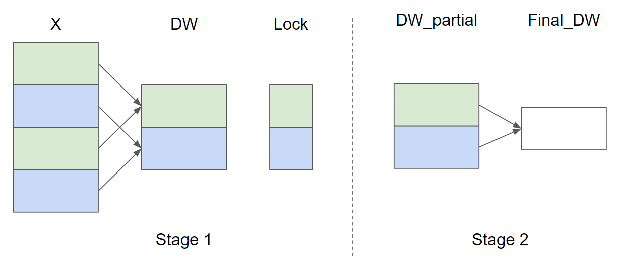
在阶段 1 中,颜色相同的 X 行共享同一个缓冲区,因此使用锁来确保在任何时候只有一个内核实例向该缓冲区写入数据。在阶段 2 中,这些缓冲区被进一步规约,以计算出最终的 \(\nabla_{w}\) 和 \(\nabla_{b}\)。在下面的实现中,阶段 1 由函数 _layer_norm_bwd_dx_fused 实现,阶段 2 由函数 _layer_norm_bwd_dwdb 实现。
@triton.jit
def _layer_norm_bwd_dx_fused(DX,  # pointer to the input gradient
                             DY,  # pointer to the output gradient
                             DW,  # pointer to the partial sum of weights gradient
                             DB,  # pointer to the partial sum of biases gradient
                             X,  # pointer to the input
                             W,  # pointer to the weights
                             Mean,  # pointer to the mean
                             Rstd,  # pointer to the 1/std
                             Lock,  # pointer to the lock
                             stride,  # how much to increase the pointer when moving by 1 row
                             N,  # number of columns in X
                             GROUP_SIZE_M: tl.constexpr, BLOCK_SIZE_N: tl.constexpr):
    # Map the program id to the elements of X, DX, and DY it should compute.
    row = tl.program_id(0)
    cols = tl.arange(0, BLOCK_SIZE_N)
    mask = cols < N
    X += row * stride
    DY += row * stride
    DX += row * stride
    # Offset locks and weights/biases gradient pointer for parallel reduction
    lock_id = row % GROUP_SIZE_M
    Lock += lock_id
    Count = Lock + GROUP_SIZE_M
    DW = DW + lock_id * N + cols
    DB = DB + lock_id * N + cols
    # Load data to SRAM
    x = tl.load(X + cols, mask=mask, other=0).to(tl.float32)
    dy = tl.load(DY + cols, mask=mask, other=0).to(tl.float32)
    w = tl.load(W + cols, mask=mask).to(tl.float32)
    mean = tl.load(Mean + row)
    rstd = tl.load(Rstd + row)
    # Compute dx
    xhat = (x - mean) * rstd
    wdy = w * dy
    xhat = tl.where(mask, xhat, 0.)
    wdy = tl.where(mask, wdy, 0.)
    c1 = tl.sum(xhat * wdy, axis=0) / N
    c2 = tl.sum(wdy, axis=0) / N
    dx = (wdy - (xhat * c1 + c2)) * rstd
    # Write dx
    tl.store(DX + cols, dx, mask=mask)
    # Accumulate partial sums for dw/db
    partial_dw = (dy * xhat).to(w.dtype)
    partial_db = (dy).to(w.dtype)
    while tl.atomic_cas(Lock, 0, 1) == 1:
        pass
    count = tl.load(Count)
    # First store doesn't accumulate
    if count == 0:
        tl.atomic_xchg(Count, 1)
    else:
        partial_dw += tl.load(DW, mask=mask)
        partial_db += tl.load(DB, mask=mask)
    tl.store(DW, partial_dw, mask=mask)
    tl.store(DB, partial_db, mask=mask)

    # need a barrier to ensure all threads finished before
    # releasing the lock
    tl.debug_barrier()

    # Release the lock
    tl.atomic_xchg(Lock, 0)


@triton.jit
def _layer_norm_bwd_dwdb(DW,  # pointer to the partial sum of weights gradient
                         DB,  # pointer to the partial sum of biases gradient
                         FINAL_DW,  # pointer to the weights gradient
                         FINAL_DB,  # pointer to the biases gradient
                         M,  # GROUP_SIZE_M
                         N,  # number of columns
                         BLOCK_SIZE_M: tl.constexpr, BLOCK_SIZE_N: tl.constexpr):
    # Map the program id to the elements of DW and DB it should compute.
    pid = tl.program_id(0)
    cols = pid * BLOCK_SIZE_N + tl.arange(0, BLOCK_SIZE_N)
    dw = tl.zeros((BLOCK_SIZE_M, BLOCK_SIZE_N), dtype=tl.float32)
    db = tl.zeros((BLOCK_SIZE_M, BLOCK_SIZE_N), dtype=tl.float32)
    # Iterate through the rows of DW and DB to sum the partial sums.
    for i in range(0, M, BLOCK_SIZE_M):
        rows = i + tl.arange(0, BLOCK_SIZE_M)
        mask = (rows[:, None] < M) & (cols[None, :] < N)
        offs = rows[:, None] * N + cols[None, :]
        dw += tl.load(DW + offs, mask=mask, other=0.)
        db += tl.load(DB + offs, mask=mask, other=0.)
    # Write the final sum to the output.
    sum_dw = tl.sum(dw, axis=0)
    sum_db = tl.sum(db, axis=0)
    tl.store(FINAL_DW + cols, sum_dw, mask=cols < N)
    tl.store(FINAL_DB + cols, sum_db, mask=cols < N)
基准测试
现在,我们可以将我们内核的性能与 PyTorch 的性能进行比较。这里我们主要关注每个特征少于 64KB 的输入。具体来说,可以通过设置 'mode': 'backward' 来对反向传播进行基准测试。
class LayerNorm(torch.autograd.Function):

    @staticmethod
    def forward(ctx, x, normalized_shape, weight, bias, eps):
        # allocate output
        y = torch.empty_like(x)
        # reshape input data into 2D tensor
        x_arg = x.reshape(-1, x.shape[-1])
        M, N = x_arg.shape
        mean = torch.empty((M, ), dtype=torch.float32, device=x.device)
        rstd = torch.empty((M, ), dtype=torch.float32, device=x.device)
        # Less than 64KB per feature: enqueue fused kernel
        MAX_FUSED_SIZE = 65536 // x.element_size()
        BLOCK_SIZE = min(MAX_FUSED_SIZE, triton.next_power_of_2(N))
        if N > BLOCK_SIZE:
            raise RuntimeError("This layer norm doesn't support feature dim >= 64KB.")
        # heuristics for number of warps
        num_warps = min(max(BLOCK_SIZE // 256, 1), 8)
        # enqueue kernel
        _layer_norm_fwd_fused[(M, )](  #
            x_arg, y, weight, bias, mean, rstd,  #
            x_arg.stride(0), N, eps,  #
            BLOCK_SIZE=BLOCK_SIZE, num_warps=num_warps, num_ctas=1)
        ctx.save_for_backward(x, weight, bias, mean, rstd)
        ctx.BLOCK_SIZE = BLOCK_SIZE
        ctx.num_warps = num_warps
        ctx.eps = eps
        return y

    @staticmethod
    def backward(ctx, dy):
        x, w, b, m, v = ctx.saved_tensors
        # heuristics for amount of parallel reduction stream for DW/DB
        N = w.shape[0]
        GROUP_SIZE_M = 64
        if N <= 8192: GROUP_SIZE_M = 96
        if N <= 4096: GROUP_SIZE_M = 128
        if N <= 1024: GROUP_SIZE_M = 256
        # allocate output
        locks = torch.zeros(2 * GROUP_SIZE_M, dtype=torch.int32, device=w.device)
        _dw = torch.zeros((GROUP_SIZE_M, N), dtype=x.dtype, device=w.device)
        _db = torch.zeros((GROUP_SIZE_M, N), dtype=x.dtype, device=w.device)
        dw = torch.empty((N, ), dtype=w.dtype, device=w.device)
        db = torch.empty((N, ), dtype=w.dtype, device=w.device)
        dx = torch.empty_like(dy)
        # enqueue kernel using forward pass heuristics
        # also compute partial sums for DW and DB
        x_arg = x.reshape(-1, x.shape[-1])
        M, N = x_arg.shape
        _layer_norm_bwd_dx_fused[(M, )](  #
            dx, dy, _dw, _db, x, w, m, v, locks,  #
            x_arg.stride(0), N,  #
            BLOCK_SIZE_N=ctx.BLOCK_SIZE,  #
            GROUP_SIZE_M=GROUP_SIZE_M,  #
            num_warps=ctx.num_warps)
        grid = lambda meta: (triton.cdiv(N, meta['BLOCK_SIZE_N']), )
        # accumulate partial sums in separate kernel
        _layer_norm_bwd_dwdb[grid](
            _dw, _db, dw, db, min(GROUP_SIZE_M, M), N,  #
            BLOCK_SIZE_M=32,  #
            BLOCK_SIZE_N=128, num_ctas=1)
        return dx, None, dw, db, None


layer_norm = LayerNorm.apply


def test_layer_norm(M, N, dtype, eps=1e-5, device=DEVICE):
    # create data
    x_shape = (M, N)
    w_shape = (x_shape[-1], )
    weight = torch.rand(w_shape, dtype=dtype, device=device, requires_grad=True)
    bias = torch.rand(w_shape, dtype=dtype, device=device, requires_grad=True)
    x = -2.3 + 0.5 * torch.randn(x_shape, dtype=dtype, device=device)
    dy = .1 * torch.randn_like(x)
    x.requires_grad_(True)
    # forward pass
    y_tri = layer_norm(x, w_shape, weight, bias, eps)
    y_ref = torch.nn.functional.layer_norm(x, w_shape, weight, bias, eps).to(dtype)
    # backward pass (triton)
    y_tri.backward(dy, retain_graph=True)
    dx_tri, dw_tri, db_tri = [_.grad.clone() for _ in [x, weight, bias]]
    x.grad, weight.grad, bias.grad = None, None, None
    # backward pass (torch)
    y_ref.backward(dy, retain_graph=True)
    dx_ref, dw_ref, db_ref = [_.grad.clone() for _ in [x, weight, bias]]
    # compare
    assert torch.allclose(y_tri, y_ref, atol=1e-2, rtol=0)
    assert torch.allclose(dx_tri, dx_ref, atol=1e-2, rtol=0)
    assert torch.allclose(db_tri, db_ref, atol=1e-2, rtol=0)
    assert torch.allclose(dw_tri, dw_ref, atol=1e-2, rtol=0)


@triton.testing.perf_report(
    triton.testing.Benchmark(
        x_names=['N'],
        x_vals=[512 * i for i in range(2, 32)],
        line_arg='provider',
        line_vals=['triton', 'torch'] + (['apex'] if HAS_APEX else []),
        line_names=['Triton', 'Torch'] + (['Apex'] if HAS_APEX else []),
        styles=[('blue', '-'), ('green', '-'), ('orange', '-')],
        ylabel='GB/s',
        plot_name='layer-norm-backward',
        args={'M': 4096, 'dtype': torch.float16, 'mode': 'backward'},
    ))
def bench_layer_norm(M, N, dtype, provider, mode='backward', eps=1e-5, device=DEVICE):
    # create data
    x_shape = (M, N)
    w_shape = (x_shape[-1], )
    weight = torch.rand(w_shape, dtype=dtype, device=device, requires_grad=True)
    bias = torch.rand(w_shape, dtype=dtype, device=device, requires_grad=True)
    x = -2.3 + 0.5 * torch.randn(x_shape, dtype=dtype, device=device)
    dy = .1 * torch.randn_like(x)
    x.requires_grad_(True)
    quantiles = [0.5, 0.2, 0.8]

    def y_fwd():

        if provider == "triton":
            return layer_norm(x, w_shape, weight, bias, eps)  # noqa: F811, E704

        if provider == "torch":
            return torch.nn.functional.layer_norm(x, w_shape, weight, bias, eps)  # noqa: F811, E704

        if provider == "apex":
            apex_layer_norm = (apex.normalization.FusedLayerNorm(w_shape).to(x.device).to(x.dtype))
            return apex_layer_norm(x)  # noqa: F811, E704

    # forward pass
    if mode == 'forward':
        gbps = lambda ms: 2 * x.numel() * x.element_size() * 1e-9 / (ms * 1e-3)
        ms, min_ms, max_ms = triton.testing.do_bench(y_fwd, quantiles=quantiles, rep=500)
    # backward pass
    if mode == 'backward':
        y = y_fwd()
        gbps = lambda ms: 3 * x.numel() * x.element_size() * 1e-9 / (ms * 1e-3)  # noqa: F811, E704
        ms, min_ms, max_ms = triton.testing.do_bench(lambda: y.backward(dy, retain_graph=True), quantiles=quantiles,
                                                     grad_to_none=[x], rep=500)
    return gbps(ms), gbps(max_ms), gbps(min_ms)


test_layer_norm(1151, 8192, torch.float16)
bench_layer_norm.run(save_path='.', print_data=True)
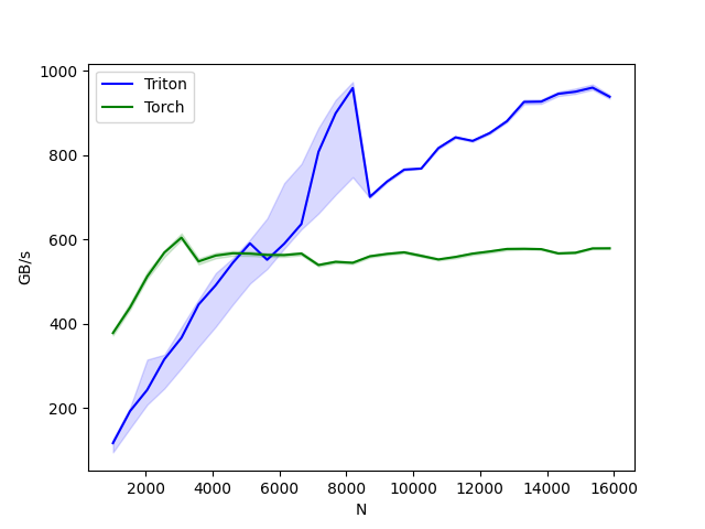
layer-norm-backward:
          N      Triton       Torch
0    1024.0  121.064037  372.363633
1    1536.0  179.824387  444.144584
2    2048.0  241.533170  517.389457
3    2560.0  337.582411  558.545450
4    3072.0  407.337026  585.142862
5    3584.0  500.093023  515.065851
6    4096.0  568.231237  522.893602
7    4608.0  582.063139  529.148312
8    5120.0  650.158735  543.716805
9    5632.0  703.999975  553.967224
10   6144.0  767.999973  563.885282
11   6656.0  840.757868  572.559140
12   7168.0  910.222229  547.872604
13   7680.0  945.230767  555.180730
14   8192.0  978.149241  561.737163
15   8704.0  694.006661  569.198909
16   9216.0  739.745803  575.999980
17   9728.0  762.980388  577.901003
18  10240.0  790.225053  579.622644
19  10752.0  784.340420  565.894726
20  11264.0  809.389194  570.329113
21  11776.0  853.848973  573.273800
22  12288.0  872.520678  583.984154
23  12800.0  887.861307  586.259571
24  13312.0  880.132233  586.216495
25  13824.0  894.274928  588.255332
26  14336.0  919.957230  576.321603
27  14848.0  952.812845  578.493529
28  15360.0  959.999966  587.006361
29  15872.0  949.945143  587.851864
参考文献
Jimmy Lei Ba and Jamie Ryan Kiros and Geoffrey E. Hinton, “Layer Normalization”, Arxiv 2016
脚本总运行时间: (0 分 29.256 秒)